Power Analyzer Automation Script
GlobTek Inc. - 2026
In order to measure the efficiency of your power supply, one might use the Yokogawa WT1800 precision power analyzer. At GlobTek we have this machine on our ATE rack, and often use it for measuing the efficiency of our power supplies. Unfortunatley, there is no straightforward way to plot the efficiency over time and plot it to Excel.
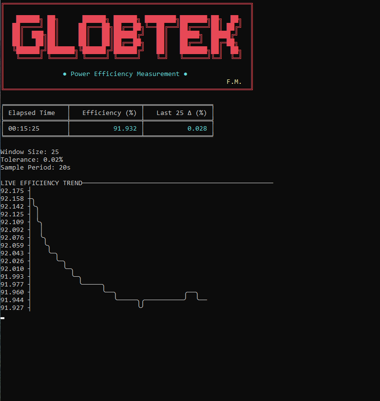
It is helpful to see the efficiency over time because when a power supply is under load, it warms up. As the components of the supply get hotter and hotter, the efficiency can either raise or lower over time (You can see this convergence in the middle image below).
Instead of recording the values by hand, I created this script to poll the instrument over GPIB, track and record a rolling window of samples, plots it in the command line, and automatically detects if the efficiency has converged.

How it works
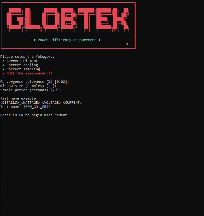
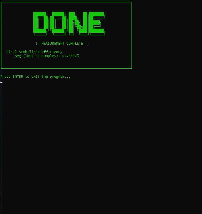
On launch, the tool asks the engineer for a convergence tolerance, sample window size, sample period, and a test name. During acquisition it shows the elapsed time, current efficiency, and the spread of the last 25 samples alongside a live ASCII trend plot. Once the efficiency falls within the set tolerance, the measurement is declared stable and the final averaged efficiency is reported.
Using PyVISA and SCPI Commands
The instrument is controlled over GPIB using PyVISA with SCPI commands from the WT1800R communication interface (NUMeric command group). After connecting and verifying the instrument with *IDN?, the script configures the analyzer’s numeric output so that a single query returns exactly the value we care about — the efficiency:
rm = pyvisa.ResourceManager()
yoko = rm.open_resource('GPIB0::21::INSTR')
yoko.query_delay = 0.5

print(yoko.query('*IDN?'))              # verify instrument identity

yoko.write(':num:num 1')                # transmit only 1 numeric item per query
yoko.write(':num:item1 ETA2,1,TOTAL')   # item 1 = efficiency η2, element 1, total order
| Command | Purpose |
|---|---|
*IDN? | IEEE 488.2 identification query - confirms the connection before measuring |
:NUMeric[:NORMal]:NUMber 1 | Sets how many numeric items VALue? transmits. The default is 15, so trimming it to 1 keeps each poll to a single clean float |
:NUMeric[:NORMal]:ITEM1 ETA2,1,TOTAL | Assigns output item 1 to the ETA2 efficiency function on element 1, TOTal order. The η2 equation itself (input vs. output power terms) is defined on the instrument via the :MEASure:EFFiciency group |
:NUMeric[:NORMal]:VALue? | Queries the configured numeric item - polled once per sample period in the main loop |
Convergence detection uses a fixed-length collections.deque as a rolling window. Each sample period, the script queries the instrument, appends the reading, and checks whether the spread of the window (max − min) is within the user-set tolerance:
data_window = collections.deque(maxlen=WINDOW_SIZE)

while True:
    eff = float(yoko.query(':NUMeric:value?'))
    data_window.append(eff)

    if len(data_window) == WINDOW_SIZE:
        data_range = max(data_window) - min(data_window)
        if data_range <= CONVERGENCE_TOLERANCE:
            break  # measurement has stabilized

    time.sleep(SAMPLE_PERIOD)
Every sample is appended to a timestamped CSV as it arrives (so no data is lost if the run is interrupted), organized into date-based folders by test name. The live terminal UI is rendered with tabulate for the stats readout and asciichartpy for the trend plot, with the last 60 samples charted in real time. When the loop exits, the final efficiency is reported as the mean of the last window:
final_avg = np.mean(full_data[-WINDOW_SIZE:])